This is the first article in a series that aims to cover common data structures.

A binary search tree is an in-memory data structure whose purpose in life is to make ultra fast searches even through large amounts of data. The main downside of this structure is the need for the data to be ordered.

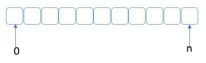
Let’s start first by identifying why a binary search is so fast. If we have an array as shown in the image below, with elements a fixed number of elements in it as long as they are sorted we can use what is called a binary search to find if an element is contained in the array or not.

A binary search purpose is to eliminate half of the data in every iteration slicing each time the amount of data that needs to be searched. In the array above, we would start by looking at the element in the middle ( n/2 ). If the data we are looking for is there our search is done. The next step is the one that makes the split it half. If the element we are looking for is less than the middle, then we repeat the search in the middle left, otherwise we repeat the search in the middle right. And then repeat the same sequence as you can see in the images below.

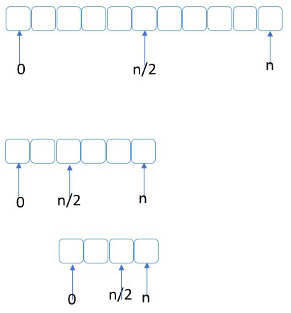
Eventually we will find the element we are looking for, or we would traverse the whole dataset in the minimum number possible of steps making sure the element is not there. Keep in mind that this algorithm takes into account the fact that the data within the array is already ordered using the same criteria that will be used to search within it. If you need to start with unsorted data, then you need to sort it first.

Now let’s take this to the next level. What if each element within the array was uniquely placed in memory with a simple way of reaching to the elements on the left, or the elements on the right? But each of those sets of elements need to maintain the same rule. That is what we can refer to as a node. A Node is going to have 3 pieces to it:

• Data
• A pointer to a node on the left
• A pointer to a node on the right

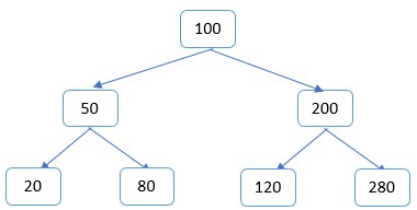
Each node will point in turn to another node, or when the node doesn’t have any left or right pointers, it is called a leaf. In the example below, you can see the node in the middle has the value of 100 - and this is called the root, because it is our entry point into the tree. All the data on the left hand side of the root is less than 100 while all the nodes on the right will have values larger than 100.

With such a tree, we can easily create a recursive search algorithm. The following piece of code is written in Java:

public class BinarySearchTree {
  //... This is a snippet
  public class Node
  {
    private Data data = NULL; // we assume Data is defined and can be compared
    private Node left = NULL;
    private Node right = NULL;

    public Node getLeft() { return left; }
    public Node getRight() { return right; }
    public Data getData() { return data; }
  }

  Node search(Node node, Data target)
  {
    if (node.getData() == target) {
      return node;
    }
    if (target < node.getData() && node.getLeft() != NULL) {
      return search(node.left, target);
    }
    if (target > node.getData() && node.getRight() != NULL) {
      return search(node.right, target);
    }
    return NULL;
  }
}

---

Below is the same approach but written in C++

struct Node
{
    Data* data; // NodeData is defined somewhere else and is comparable
    Node* left = NULL;
    Node* right = NULL;
};

Node* search(Node *node, Data &target)
{
  if (!node) {
    return NULL;
  }
  if (*node->data == target) {
    return node;
  }
  if (target < *node->data && node->left) {
    return search(node->left, target);
  }
  if (target > *node->data && node->right) {
    return search(node->right, target);
  }
  return NULL;
}

Stay tuned, because in future articles I will add more operations to the Binary Search Tree and will also talk about optimizing the code utilizing more object oriented principles and strengths of Java and C++.